Predicted CLV model

Predicted customer lifetime value predicts the total value of all orders a customer is likely to make if they return to make another purchase during the next 365 days.

About predicted CLV models

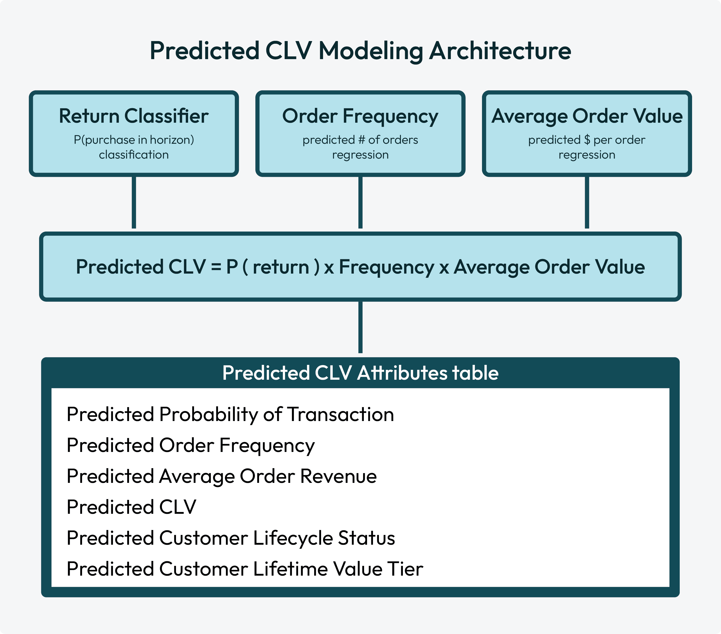
The predicted CLV model predicts the expected revenue for each customer, likelihood of purchasing, and their value relative to other customers over a future time window (the “prediction horizon,” typically the next 365 days). Rather than relying on a single model for this complex prediction, pCLV breaks the problem into three simpler, independently trained machine learning models that are then combined to produce the final prediction.

A customer’s future value is a function of three questions:

1. Will they come back? The Return Classifier predicts the probability that a customer will make at least one purchase during the prediction horizon.

2. How often will they buy? The Order Frequency Regressor predicts how many orders a returning customer will place during the prediction horizon.

3. How much will they spend per order? The Average Order Value Regressor predicts the average revenue per order for the customer.

How predicted CLV works

The predicted CLV model is an ensemble learning method with three independently trained submodels: a return classifier, an order frequency regression, and an average order value regression. Each individual model contributes independently to the predicted CLV model’s output: predicted CLV scores.

Return classifier

The return classifier submodel predicts the probability that a customer will make at least one purchase during the prediction horizon. This is a binary classification: will a customer return or not return? The prediction is output as a probability score between 0 and 1.

Note

Customers with a very low return probability will naturally have a low predicted CLV regardless of other factors.

Order frequency regression

The order frequency regression submodel predicts how many orders a returning customer will place during the prediction horizon, and then outputs a continuous number. For example: 3.2.

Average order value regression

The average order value regression submodel predicts the average revenue per order for the customer, and then outputs a dollar amount. For example: “$85.40”.

Predicted CLV scores

The return classifier, order frequency regression, and average order value regression submodels are combined with a multiplicative ensemble:

Predicted CLV = P(return) x Predicted Order Frequency x Predicted Avg Order Value

A customer with a high probability of return but low order frequency and modest order value will have a moderate CLV, while a customer who is likely to return frequently and spend heavily will have a high CLV.

After raw scores are computed, a sigmoid rescaling step compresses extreme outlier predictions to produce a smoother distribution of values.

Use predicted CLV modeling to build high-value audiences that identify:

• Which customers have the highest predicted value?

• Which customers are better candidates for winback offers?

• Which customers are candidates for cultivating customer value?

Use cases

The predicted CLV model helps you identify your highest value customers by year or by value tier:

1. How much will customers spend in the next year?

2. Which customers are your most valuable customers?

How much will customers spend?

The Predicted CLV Next 365 Days attribute in the Predicted CLV Attributes table contains the total predicted customer spend over the next 365 days. You can access this attribute directly from the Segment Editor.

After you select this attribute you can specify the type of values you want to use for this audience, such as:

• Predicted CLV is greater than $100

• Predicted CLV is less than $400

• Predicted CLV is between $100 and $400

Which customers are the most valuable?

When predictive modeling is enabled for your tenant you can use output from the predicted customer lifetime value (CLV) model, which helps you identify your highest value customers by value tier. Each tier represents a percentile grouping of customers by predicted value:

• Platinum represents the top 1%

• Gold represents customers who fall between 1% and 5%

• Silver represents customers who fall between 5% and 10%

Select all three of these predicted value tiers to build an audience that contains customers who are predicted to be in your top 10% (inclusive) high value customers.

Build a predicted CLV model

You can build a predicted CLV model from the Customer 360 page. Any database that contains the Merged Customers, Unified Itemized Transactions, and Unified Transactions tables may be configured for predictive modeling.

Important

The following fields are automatically included in all predictive models:

Table	Fields
Merged Customers	Predictive models always use the following fields in the Merged Customers table: Amperity ID Birthdate City Email Gender Given name Phone Postal State Surname
Unified Transactions	Predictive models always use the following fields in the Unified Transactions table: Amperity ID Order datetime Order ID Order quantity Order revenue The following fields, when they are available in the Unified Transactions table, will also be used: Order cancelled quantity Order cancelled revenue Order discount amount If your tenant does not have order-level discount data, define order-level discounts to equal the sum of item-level discount amounts. This will ensure that predictive modeling is able to incorporate signals for discount shoppers. Order returned quantity Order returned revenue Purchase brand Purchase channel Store ID
Unified Itemized Transactions	Predictive models always use the following fields in the Unified Itemized Transactions table: Amperity ID Is return Item quantity Item revenue Order datetime Order ID Product ID

To build a predicted CLV model

1. Select model, create version

2. Choose lookback window

3. Configure global hyperparameters

4. Configure hyperparameters for submodels

5. Evaluate versions

6. Choose version

Select model, create version

Open the Customer 360 page and select a database. Click the menu to open the menu, and then select Predictive models. This opens the Predictive models page.

Click the Add model button and select Predicted customer lifetime value (pCLV). In the New model dialog assign a name to the model and add a description.

From the Prediction horizon dropdown select the number of days into the future for which predictions are made: 90 days, 180 days, or 365 days (default).

Choose lookback window

The lookback window defines the number of years of historical data to use for training the predicted CLV model. Choose one of 4 years, 5 years, or 6 years.

Configure global hyperparameters

Select the Advanced tab to configure the global hyperparameters.

Important

Global hyperparameters for predicted CLV modeling are only configurable during initial version setup.

Max training size defines the maximum number of customer records to use when training the model. Larger values increase processing time.

Enable Balance labels to downsample the majority class and upsample the minority class.

Enable Filter outliers to exclude outliers from model training.

Use the Customer exclusions dropdown to configure a list of fields from the Customer Attributes table. Customer profiles that match a selected field from the Customer Attributes table are excluded from predictive CLV modeling output.

Configure hyperparameters for submodels

Hyperparameters for submodels are configured from the Advanced tab. Expand Predicted probability of transaction, Predicted order frequency, and Predicted average order value to configure hyperparameters for each submodel. When finished, click Evaluate.

Important

Hyperparameters for submodels are only configurable during initial version setup.

Components of predictive CLV modeling have the following hyperparameters:

Parameter	Default	Description
Elastic net parameter	0.0	Applies to Logistic regression model types. Controls the mixing ratio for L1 regularization, also known as LASSO , and L2 regularization, also known as ridge regression applied to elastic net regression . Range: 0.0 to 1.0. A value of “0.0” applies only L2 regularization. Weights are penalized proportional to their square, which shrinks weights toward zero. Values between 0.0 and 1.0 blend L1 and L2 regularization. A value closer to “0.0” encourages a smaller and more even distribution of weights. A value closer to “1.0” leads to sparse models. A value of “1.0” applies only L1 regularization. Weights are penalized proportional to their absolute value.
Feature subset strategy	Auto	Applies to Random forest and Gradient boosted trees model types. The random forest model is intentionally trained on a random subset of features at each split to ensure that each tree within the random forest is different. The value for Feature subset strategy determines how features are split into random subsets. Possible values: Strategy Description All All features are in all splits. Use only for small feature sets or to ensure random forest classifier outputs are not random. Auto Default. Allow the random forest classifier to choose the feature subset strategy. Log2 Use a base 2 binary logarithm to determine the split. For example, if there are 100 features, the split is ~7. One third Use one third of features to determine the split. For example, if there are 100 features, the split is 33. Square root Use the square root of features to determine the split. For example, if there are 100 features, the split is 10.
Fit intercept	Enabled	Applies to Logistic regression model types. Enable Fit intercept to include a bias term, which is a constant added to predictive CLV modeling regardless of feature values. When Fit intercept is disabled the predictive CLV modeling predicts zero when all features are zero.
Impurity	Gini	Applies to Random forest model types for the Predicted probability of transaction submodel. The predictive CLV model uses impurity to evaluate the quality of a candidate split at each node. For example: “Customers with more than 3 orders in the last 90 days” go into one branch of the split and “Everyone else” goes into the other. Impurity measures if the split produces more homogenous groups than the parent node did. A good split pushes customers who will return into one branch and customers who won’t into the other. The predictive CLV model picks the branch with the greatest reduction in impurity. Use “Gini” to measure the probability of misclassifying a randomly chosen customer. Gini favors splits that isolate the single largest class and is well-suited for imbalanced datasets where non-returners significantly outnumber returners. Use “Entropy” to measure the average amount of information needed to describe a randomly chosen customer. Entropy produces more balanced splits and finds patterns when returners contain meaningful subgroups.
Loss type	Squared	Applies to Gradient boosted trees model types. Defines what is minimized by a model during training. Use “Squared” to minimize mean squared errors common to predicting order frequency and average order value. Squared can be sensitive to large errors from outlier orders. Use “Absolute” to minimize mean absolute errors. For Predicted order frequency and Predicted average order value submodels switch from “Squared” to “Absolute” when average order value or order frequency data has extreme high-value outliers that distort predictions.
Max bins	102	Applies to Gradient boosted trees and Random forest model types. The maximum number of bins for discretization of continuous features . Before a tree is split on a continuous feature the random forest model must decide where to try splitting. This setting defines the maximum number of candidate thresholds within a dataset the random forest model is allowed to evaluate before splitting data. For example, with a very low number of bins, such as 10, the random forest model may try for ten evenly spaced splits. More bins gives the random forest model more ways to find precise splits. Max bins is the maximum number of bins available. Some values are grouped together when the number of possible splits exceeds the maximum number of bins. Range: 2 to 256. If a feature has fewer unique values than the Max bins value, the bin count is irrelevant. The random forest model evaluates every unique value as a candidate for splitting. The Max bins value constrains features with high cardinality or features that are truly continuous. Setting Max bins to 256 for a feature with 12 unique values results in 12 candidates for splitting.
Max depth	10	Applies to Gradient boosted trees and Random forest model types. The maximum depth of each tree in the random forest classifier. Range: 1 to 30. This setting controls the levels of splits a tree is allowed to make. At each level a yes/no question is asked and, depending on the answer, the data is split into two groups. For example: Tree: Age > 30? |__ Yes. Purchases > 3? < depth 1 | |__ Yes. Socks? < depth 2 | | |__ Yes. Brand = Socktown? < depth 3 | | | |__ Yes. < depth 4 | | | | |__ Yes. Color = blue? < depth 5 | | | | |__ No. < depth 5 | | | | | | | |__ No. < depth 4 | | | | | |__ No. < depth 3 | | | |__ No. < depth 2 | |__ No. < depth
Max iterations	100	Applies to Gradient boosted trees and Logistic regression model types. The maximum number of sequential boosting rounds. Each boosting round fits a new tree to correct residual errors for all previous trees. More iterations allow more training data to be fit more precisely. Range: 1 to 1000 for Logistic regression models and 1 to 500 for Gradient boosted trees models. Tip Modify the values of Max iterations and Step size together. A smaller step size requires more iterations. When a predictive CLV model is underfitting increase the value of Max iterations and decrease the value of Step size.
Min info gain	0	Applies to Random forest model types. The minimum information gain required for a split. A split is only made when it reduces Impurity by at least the value of Min info gain. At zero the model considers every possible split regardless of improvement and produces more complex trees. A value greater than zero prunes away weak splits early and leads to less complex trees that train faster and generalize better. Increase this value to limit tree depth when training contains low-value splits.
Min instances per node	1	Applies to Gradient boosted trees and Random forest model types. The minimum number of training instances required before a leaf node split is allowed. Increase this value when training data has a long tail of unusual customers, the predictive CLV model overfits, or when predictions are based on broad patterns instead of individual behavior.
Model type	Random forest	All models have Gradient boosted trees and Random forest options. The Predicted probability of transaction model has an option for Logistic regression. A Random forest model builds many independent decision trees and averages their predictions. A Gradient boosted trees model builds trees sequentially, with each new tree correcting the errors of the previous ones. Can be more powerful than a Random forest model, but is more sensitive to tuning. A Logistic regression model predicts probabilities by fitting a linear decision boundary through a sigmoid function. A Logistic regression model is faster to train than tree-based models and is more interpretable, but less able to capture complex nonlinear patterns.
Number of trees	100	Applies to Random forest model types. The number of individual trees available to the random forest classifier. More trees create more stable and more accurate random forest classifier outcomes. Start with 100 trees and increase or decrease this number during model evaluation to determine which number creates the best outcomes. The maximum number of trees is 500.
Regularization	0.0	Applies to Logistic regression model types. The strength of the regularization penality applied to coefficient weights. Higher values push weights closer to zero and prevent predictive CLV modeling from relying too heavily on any single feature. Increase this value to reduce overfitting. Range: 0.0 or greater.
Standardize features	Enabled	Applies to Logistic regression model types. Enable Standardize features to rescale each feature to have zero mean and zero unit variance before training. Standardizing features ensures regularization is applied evenly across all features. Only disable Standardize features when features are already standardized upstream or if feature scale carries meaningful signal you don’t want removed.
Step size	0.1	Applies to Gradient boosted trees model types. The learning rate. At each boosting round a tree’s contribution is scaled by the value of Step size, after which the tree is added to the ensemble. A smaller step size leads to more cautious models. Each tree has less influence. More trees are required. A larger step size converges faster, but at the risk of overfitting. Range: 0.01 to 1.0. The default value is a conservative starting point. Decrease this value to improve model quality at the cost of longer training times.
Subsampling rate	1.0	Applies to Gradient boosted trees and Random forest model types. The fraction of training records randomly sampled without replacement when building each tree. The range for this value is between 0.1 and 1.0. At 1.0 every tree sees the full training set. Values below 1.0 ensure each tree sees a different subset and ensure random sampling among trees.

Evaluate versions

Each version must be evaluated before it can be selected for use with predicted CLV modeling.

Metric	Description
Architecture	The combination of models used by the submodels of predictive CLV modeling displayed as a slash-separated abbreviated string in the following order: return classifier / order frequency regression / average order value regression. RF is random forest GBT is gradient boosted trees LR is logistic regression For example: RF/RF/RF.
Brier score	A Brier score measures prediction accuracy for the return classifier submodel and displays as an improvement percentage relative to a 90-day naive baseline. A lower score is better.
Evaluation	Did model evaluation pass or fail?
Last ran	The date and time at which the model’s validation run completed.
Lookback window	The number of years of historical transaction data used to train the predicted CLV model.
MAE	Mean absolute error (MAE) measures the average dollar error between predicted CLV and actual CLV across all customers. MAE shows the percentage improvement over baseline and displays as actual versus predicted average spend amounts. A lower value is better. A large value indicates imprecise predictions even if rankings are good.
Spearman’s rank	A Spearman’s rank measures how well a model ranks customers by predicted lifetime value relative to their actual lifetime value and displays as an improvement percentage over a naive baseline ranking. A higher value is better and indicates a greater percentage of high-value customers who are predicted to purchase.
Status	The current state of the model version’s training and evaluation run.

Choose version

Choose the version that performs best for predicted CLV modeling, and then click the Edit button.

On the Schedule page:

1. Set Status to Active.

   Important

   Only activate a version that performs best for your marketing use cases.

2. From the Courier group dropdown select a courier group. Active predicted CLV models must be attached to a courier group.

3. Inference cadence is the frequency at which predictions are generated. Under Inference refresh set the frequency. The default value is 1, which refreshes predictions daily.

4. Training cadence is the frequency at which predicted CLV modeling is retrained with new data. Under Training refresh set the frequency. The default value is 14, which retrains with new data every two weeks.

5. Click Save to activate the predicted CLV model. A full workflow starts that trains the model, runs inference, and then adds predicted CLV output tables to the database.

Predicted CLV output tables

The Predicted CLV Attributes table has the output of predicted CLV modeling.

Note

Field names use “365d” as the default prediction horizon. If a predicted CLV model uses a different prediction horizon, such as “90 days” or “180 days”, column names in the database table are not updated. The data in the table rows always matches the value for the lookback window.

The Predicted CLV Attributes table has the following columns:

Column name	Data type	Description
Amperity ID	String	The unique identifier assigned to clusters of customer profiles that all represent the same individual. The Amperity ID does not replace primary, foreign, or other unique customer keys, but exists alongside them within unified profiles. Note The Amperity ID is a universally unique identifier (UUID) that is 36 characters spread across five groups separated by hyphens: 8-4-4-4-12. For example: 123e4567-e89b-12d3-a456-426614174000
Days Since Last Order	Integer	The number of days elapsed since the customer’s last order.
Historical Order Frequency Lifetime	Integer	The total number of historical orders a customer has made.
Predicted Average Order Revenue Next 365D	Decimal	The predicted average order revenue over the next 365 days.
Predicted CLV Next 365D	Decimal	The total predicted customer spend over the next 365 days.
Predicted Customer Lifecycle Status	String	A probabilistic grouping of a customer’s likelihood for future transactions. For repeat customers, groupings include the following tiers: Active Likelihood to purchase is greater than 60%. Cooling down Likelihood to purchase is between than 50% and 60%. At risk Likelihood to purchase is between than 35% and 50%. Highly at risk Likelihood to purchase is between than 20% and 35%. Lost Likelihood to purchase is less than 20%. For one-time buyers, groupings include the following tiers: Active Purchased within 60 days. Cooling down Purchased 60-120 days ago. At risk Purchased 120-180 days ago. Highly at risk Purchased 180-240 days ago. Lost Purchased 240+ days ago.
Predicted Customer Lifetime Value Tier	String	A percentile grouping of customers by predicted CLV. Groupings include: Platinum: top 1% of customers Gold: top 1%-5% of customers Silver: top 5%-10% of customers Bronze: top 10%-25% of customers Medium: top 25%-50% of customers Low: bottom 50% of customers Note This attribute returns only the customers who belong to the selected value tier. For example, to return all of your top 10% customers, you must choose platinum, gold, and silver. Silver by itself will return 5% of your customers, specifically those are in your 5-10%.
Predicted Order Frequency Next 365D	Decimal	The predicted number of orders over the next 365 days.
Predicted Probability Of Transaction Next 365D	Decimal	The probability a customer will purchase again in the next 365 days.

Export validation results

Export model results to Databricks, Google BigQuery, or Snowflake using an outbound bridge.

Configure an outbound bridge, and then select the predictive_tables dataset. The validation export includes actual customer spend and churn status for all customers in the holdout dataset and the scores from the model and comparison baseline.

Column name	Description
amperity_id	The unique customer identifier.
predicted_probability_of_transaction_next_365d	The predicted likelihood (0-1) of a customer transacting in the prediction horizon.
predicted_order_frequency_next_365d	Assuming a customer will transact, the predicted number of orders they will make in the prediction horizon.
predicted_average_order_revenue_next_365d	Assuming a customer will transact, the predicted average value per order for any orders in the prediction horizon.
predicted_clv_next_365d	The total predicted spend over the prediction horizon, calculated as predicted_probability_of_transaction_next_365d * predicted_order_frequency_next_365d * predicted_average_order_revenue_next_365d.
historical_order_frequency_lifetime	The customer’s lifetime number of orders as of the start of the evaluation window.
days_since_last_order	The days since the customer’s last order, as of the start of the evaluation window.
naive_predicted_clv_next_365d	The total expected spend over the prediction horizon, using the naive baseline. The baseline carries forward a customer’s spend during the preceding period equal to the prediction horizon and assumes they will do the same in the prediction horizon.
predicted_customer_lifecycle_status	Customer lifecycle segment: Lost, Highly at risk, At risk, Cooling down, or Active.
predicted_customer_lifetime_value_tier	Value tier based on CLV percentile: Low, Medium, Bronze, Silver, Gold, or Platinum.
_actual_returned	The customer’s actual transaction status in the evaluation window. 1 for return, 0 for churn.
_actual_order_freq	The customer’s actual order amount in the evaluation window.
_actual_average_order_value	The customer’s actual average order value in the evaluation window.
_actual_clv	The customer’s actual spend in the evaluation window.