Build queries¶

A query is SQL that runs from the Queries page against database tables in the Customer 360 page. A query returns a refined and filtered subset of useful customer data.

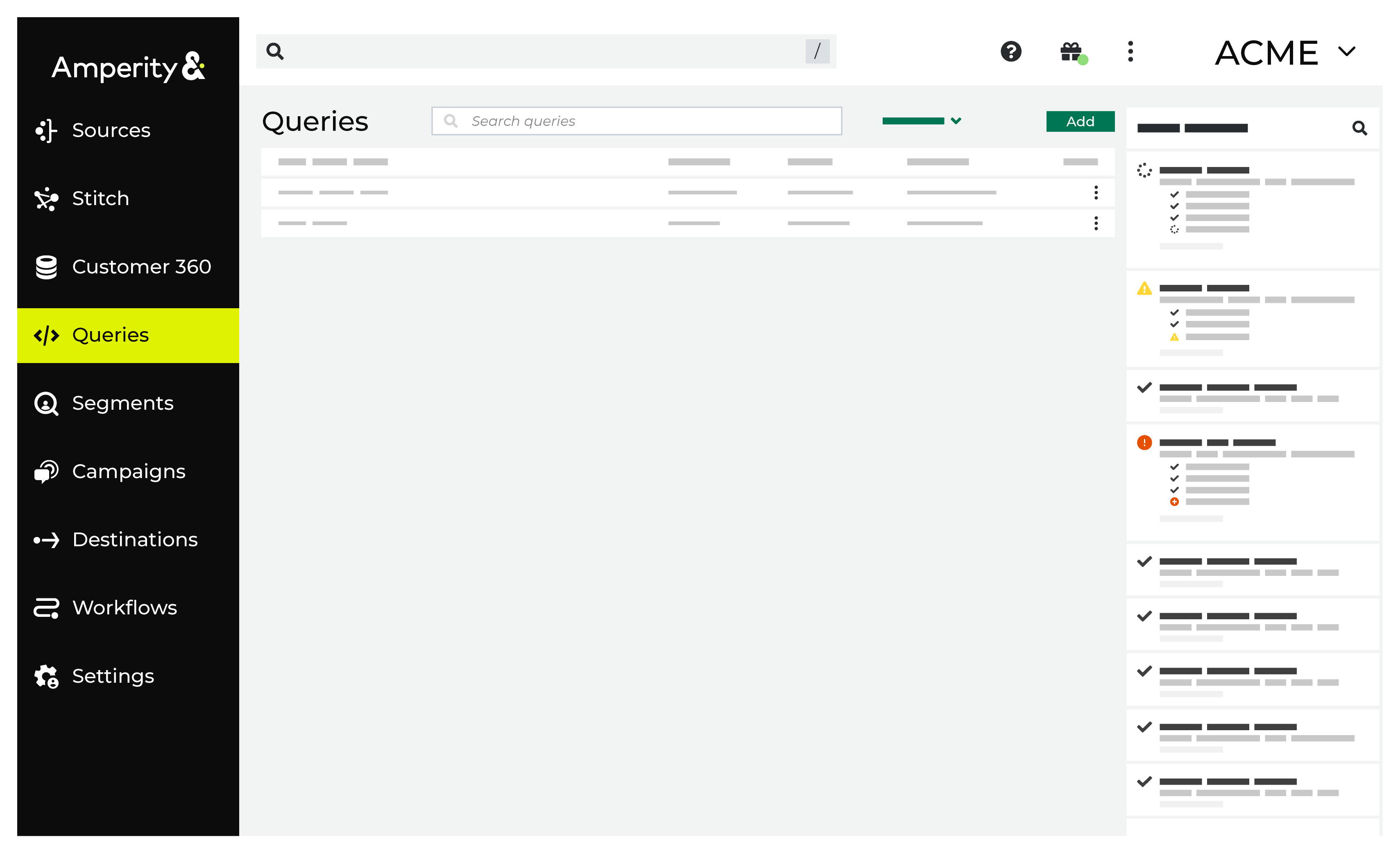
Queries page¶

The Queries page provides an overview of the status of every query. A table shows the status and details. Queries are listed by row. The details include the date and time at which this query last ran, along with the number of records (rows) that were returned during the last completed run.

Query editor¶

The SQL Query Editor is the user interface for a full SQL query engine based on Presto SQL that interacts with customer database tables in Amperity. The SQL Query Editor relies primarily on using the SELECT statement, along with common table expressions, joins, functions, and other parts of Presto SQL to build and design advanced queries.

Use the Query Editor to build SQL queries against tables and columns in your customer 360 database to support any downstream workflow. The Query Editor uses Presto SQL.

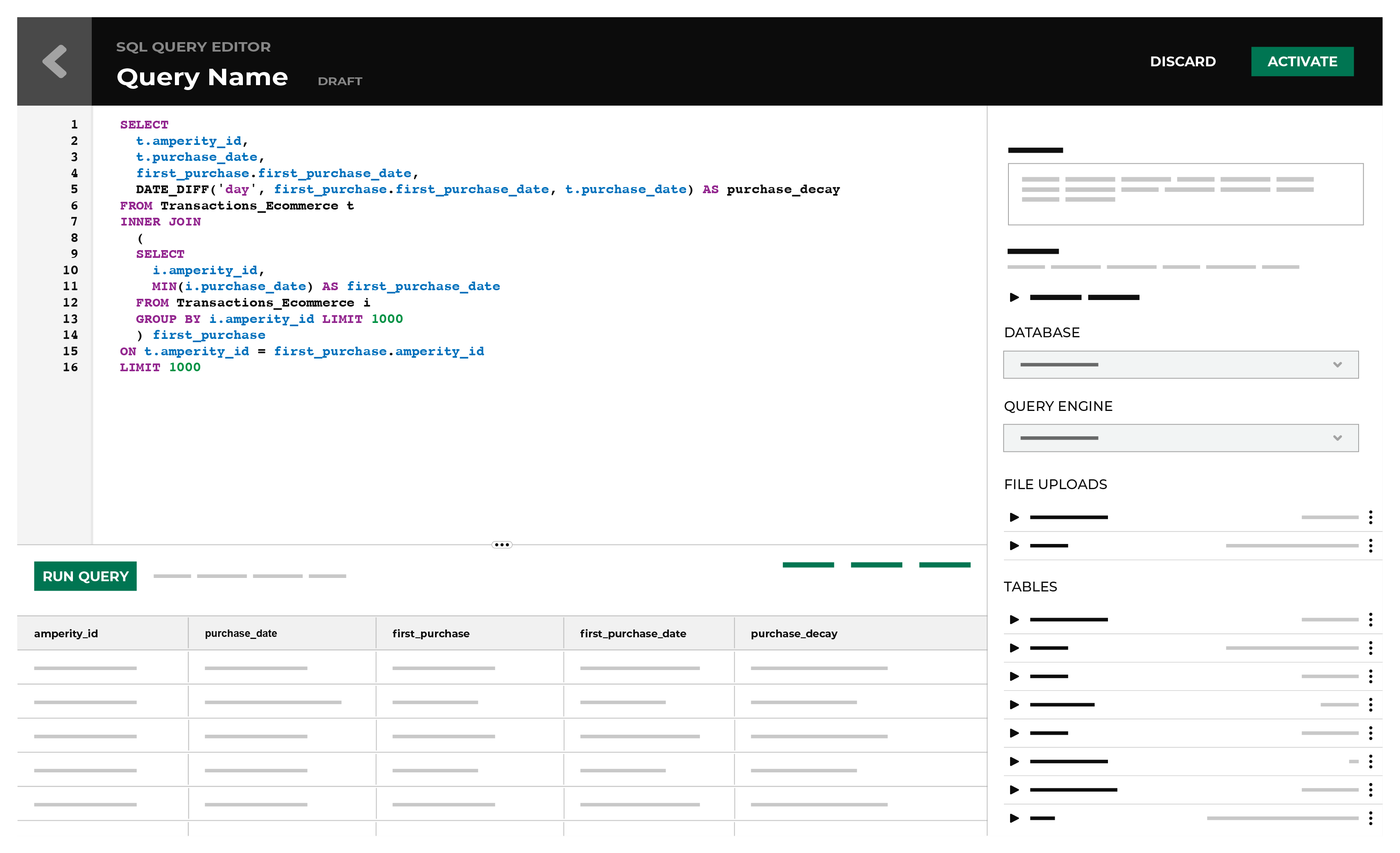
Use the SQL Segment Editor on the Queries page.

Queries may be authored using the visual Query Editor or the SQL Query Editor. Click Create, and then select the query editor to open. Queries that are already created have an icon that shows from which query editor they were authored.

indicates the query was created using the visual Query Editor.
indicates the query was created using the SQL Query Editor.

All queries must be activated before they can run as part of a scheduled workflow.

Note

Amperity is a multi-user system and the set of queries for your company is shared across all users. That means that if one user creates a draft query, another can open and edit it, so work can be easily passed between people on your team.

However, it also means that if 2 users are editing the same thing at the same time, their changes will collide. Amperity resolves this by applying the last set of changes saved as a whole. This will always keep the query in a consistent state (it will never be half-implemented). But changes that were saved first will be overwritten. As a result, we strongly recommend that you coordinate changes to specific objects in Amperity with others on your team.

About Presto SQL¶

Presto is a distributed SQL query engine designed to efficiently query large amounts of data using distributed queries. The Queries and Segments pages use Presto to return query results and audience segments.

Amperity queries are built using Presto SQL to define a SELECT statement. Please refer to the Presto SQL reference.

All queries that are built via the SQL Query Editor are done using a SELECT statement. In some cases, a WITH is used along with the SELECT statement. Each select statement can additional functionality, such as WHERE, LEFT JOIN, GROUP BY, ORDER BY, LIMIT clauses, CASE expressions, functions, operators, and other components that are part of Presto SQL, which is the underlying SQL engine for both the visual Query Editor and SQL Query Editor.

Tip

Follow the recommendations and patterns for indentation, naming conventions, reserved words, and whitespace.

Build queries¶

Queries may be authored using the visual Query Editor or the SQL Query Editor. Click Create and then select the query editor to open. Queries that are already created have an icon that shows from which query editor they were authored. All queries must be activated before they can run as part of a scheduled workflow.

Add query¶

To add a query using the SQL Query Editor

From the Queries page click Create, and then select SQL Query. This opens the SQL Query Editor.
Under Database, select a database. The Customer 360 database is selected by default.
Define the query against the selected database.
Click Run Query and debug any issues that may arise.
Click Activate.

Preview results¶

You can preview the results of a SQL query by clicking the Run Query button. This will do one of the following things:

Return the first 100 results of the query to the preview pane directly below the query editor.
Return an empty table.
Return some type of error.

Use the preview results pane to fine-tune your queries, to make sure they return the data you want, and to make sure they don’t contain any errors.

Tip

Query editor SQL queries often evaluate millions of records. This means they may take a few minutes to run. You may use other areas of Amperity while a query is being run.

For draft queries, setting a the LIMIT clause to “100” while developing a query is often enough for testing and validating query results against very large data sets.

To preview query results

From the Queries page, open the menu for a query, and then select View. This opens a query editor.
Click Run Query to run the query. Wait for it to return results.
Example the columns and the data that is in them.
Adjust your query as necessary until it runs correctly.
Click Activate.

Validate query¶

SQL queries are validated from the SQL Query Editor by clicking the Run Query button. The results of the query are returned in the results window. The quality of the results can be inspected, and then fine-tuned. Errors in the syntax are reported in the results window.

Add to orchestration¶

Use the Orchestration option to define a schedule for a query.

To add a query to an orchestration

From the Queries page, open the menu for a query, and then select View. This opens a query editor.

Tip

The query does not need to be in edit mode to configure an orchestration.
Under Being Sent To click Add one now. This opens the Add Orchestration dialog box.
Follow the steps to add an orchestration. The steps will vary depending on the destination, the data template, and the orchestration.
Click Save.

Example queries¶

This section contains examples of queries that you can add to your tenant:

Important

These queries are not meant to be copy/paste queries. Use them as examples. Most will require some customization to be used effectively within your tenant.

Cohort analysis¶

The following SQL builds a cohort analysis against the Transaction Attributes Extended table that returns a month-by-month view of customers acquired, split by channel (store vs. online), and then for each monthly cohort, how many repurchased within 60, 90, 180, and 365 days, and the channel on which customers made their repeat purchases.

Tip

Build cohort analysis queries for your tenant, and then send the results downstream to your favorite analytics and/or BI tool.

SELECT
  YEAR(tae.first_order_datetime) AS first_order_year
  ,MONTH(tae.first_order_datetime) AS first_order_month
  ,tae.first_order_purchase_channel
  ,COUNT(*) AS num_amp_id
  ,SUM(CASE
    WHEN tae.second_order_datetime <= tae.first_order_datetime + interval '60' day
    THEN 1
    ELSE 0
  END) AS repeat_60d
  ,SUM(CASE
    WHEN tae.second_order_purchase_channel = 'web'
    AND tae.second_order_datetime <= tae.first_order_datetime + interval '60' day
    THEN 1
    ELSE 0
  END) AS repeat_60d_web
  ,SUM(CASE
    WHEN tae.second_order_purchase_channel = 'store'
    AND tae.second_order_datetime <= tae.first_order_datetime + interval '60' day
    THEN 1
    ELSE 0
  END) AS repeat_60d_store
  ,SUM(CASE
    WHEN tae.second_order_purchase_channel = 'web'
    AND tae.second_order_datetime <= tae.first_order_datetime + interval '90' day
    THEN 1
    ELSE 0
  END) AS repeat_90d_web
  ,SUM(CASE
    WHEN tae.second_order_purchase_channel = 'store'
    AND tae.second_order_datetime <= tae.first_order_datetime + interval '90' day
    THEN 1
    ELSE 0
  END) AS repeat_90d_store
  ,SUM(CASE
    WHEN tae.second_order_purchase_channel = 'web'
    AND tae.second_order_datetime <= tae.first_order_datetime + interval '180' day
    THEN 1
    ELSE 0
  END) AS repeat_180d_web
  ,SUM(CASE
    WHEN tae.second_order_purchase_channel = 'store'
    AND tae.second_order_datetime <= tae.first_order_datetime + interval '180' day
    THEN 1
    ELSE 0
  END) AS repeat_180d_store
  ,SUM(CASE
    WHEN tae.second_order_purchase_channel = 'web'
    AND tae.second_order_datetime <= tae.first_order_datetime + interval '365' day
    THEN 1
    ELSE 0
  END) AS repeat_365d_web
  ,SUM(CASE
    WHEN tae.second_order_purchase_channel = 'store'
    AND tae.second_order_datetime <= tae.first_order_datetime + interval '365' day
    THEN 1
    ELSE 0
  END) AS repeat_365d_store
FROM Transaction_Attributes_Extended tae
GROUP BY 1,2,3
ORDER BY 1,2,3

Count loyalty by state¶

The following example counts customers in the United States, and then also in California, Oregon, Washington, Alaska, and Hawaii who also belong to the loyalty program (which is indicated when loyalty_id is not NULL):

SELECT
  state
  ,COUNT(amperity_id) AS TotalCustomers
FROM
  Customer360
WHERE (UPPER("country") = 'US'
AND UPPER("state") in ('AK', 'CA', 'HI', 'OR', 'WA')
AND LOWER("loyalty_id") IS NOT NULL)
GROUP BY state

Customer acquisition¶

The following examples show how to track customer acquisition by day for single- and multi-brand tenants.

Tip

Build customer acquisition queries for your tenant, and then send the results downstream to your favorite analytics and/or BI tool.

For single-brand tenants

SELECT
  DATE(first_order_datetime) AS first_order_date
  ,COUNT(DISTINCT amperity_id) AS total_customers
  ,SUM(CASE
    WHEN one_and_done
    THEN 1
    ELSE 0
  END) AS total_one_and_done
  ,AVG(lifetime_order_revenue) AS avg_clv
  ,SUM(CASE
    WHEN L12M_order_frequency > 0
    THEN 1
    ELSE 0
  END) AS L12M_total_orders
FROM Transaction_Attributes_Extended
GROUP BY 1,2,3
ORDER BY 1,2,3

For multi-brand tenants

SELECT
  multi_purchase_brand
  ,multi_purchase_channel
  ,DATE(first_order_datetime) AS first_order_date
  ,COUNT(DISTINCT amperity_id) AS total_customers
  ,SUM(CASE
    WHEN one_and_done
    THEN 1
    ELSE 0
  END) AS total_one_and_done
  ,AVG(lifetime_order_revenue) AS avg_clv
  ,SUM(CASE
    WHEN L12M_order_frequency > 0
    THEN 1
    ELSE 0
  END) AS L12M_total_orders
FROM Transaction_Attributes_Extended
GROUP BY 1,2,3
ORDER BY 1,2,3

Days to second purchase¶

The following example shows how to return the days to second purchase starting from a date range for the first order.

SELECT
  days_to_second_purchase
  ,COUNT(DISTINCT amperity_id) AS "customer_count"
FROM (
  SELECT
    amperity_id
    ,first_order_datetime
    ,second_order_datetime
    ,DATE_DIFF('day', first_order_datetime, second_order_datetime) AS "days_to_second_purchase"
  FROM Transaction_Attributes_Extended
  WHERE (
    (
      "amperity_id" IN (
        SELECT DISTINCT "t0"."amperity_id"
        FROM "Transaction_Attributes_Extended" "t0"
        WHERE (
          "t0"."first_order_datetime" BETWEEN TIMESTAMP '2019-01-01'
          AND TIMESTAMP '2022-01-01'
          AND "t0"."second_order_datetime" IS NOT NULL
        )
      )
    )
  )
  GROUP BY amperity_id, first_order_datetime, second_order_datetime
)
GROUP BY 1
ORDER BY 1 ASC

Tip

You can extend the WHERE statement to show days to second purchase by brand:

WHERE (
  "t0"."first_order_datetime" BETWEEN timestamp '2019-12-01'
  AND timestamp '2023-12-28'
  AND "t0"."second_order_datetime" IS NOT NULL
  AND "t0"."first_order_purchase_brand" = 'Brand A'
  --AND "t0"."first_order_purchase_brand" = 'Brand B'
  --AND "t0"."first_order_purchase_brand" = 'Brand C'
  --AND "t0"."first_order_purchase_brand" = 'Brand ...'
  --Comment brands out when not needed
)

Google Analytics reports¶

The following example shows how build acquisition channel reports using the GoogleAnalytics4_TransactionalAnalytics4 table that is created by the Google Analytics data source.

WITH first_order AS (
  SELECT DISTINCT
    ut.amperity_id
    ,order_ID
    ,first_order_datetime
  FROM Unified_Transactions ut
  INNER JOIN (
    SELECT
      amperity_id
      ,first_order_datetime
    FROM Transaction_Attributes_Extended
    WHERE first_order_datetime
    BETWEEN timestamp '2022-09-05 00:00:00'
    AND timestamp '2022-09-13 00:00:00') ta
  ON ta.amperity_id = ut.amperity_id
  AND ta.first_order_datetime = ut.order_datetime
)

SELECT
  sessionSource
  ,COUNT(amperity_id) new_customers
FROM first_order
LEFT JOIN (
  SELECT
    transactionId
    ,sessionSource
  FROM GoogleAnalytics4_TransactionalAnalytics4
) GA
ON first_order.order_ID = GA.transactionId
GROUP BY 1
ORDER BY 2 DESC

What columns are available?

You can use any column in the GoogleAnalytics4_TransactionalAnalytics4 table to build reports:

itemRevenue
transactionId
browser
sessionCampaignName
sessionSource
sessionGoogleAdsAdGroupName
date
deviceCategory
operatingSystem
sessionGoogleAdsQuery
operatingSystemVersion
sessionMedium
sessionGoogleAdsAdGroupId

Leaky bucket ratio¶

A leaky bucket ratio tracks the difference between the customers your brand wins and loses over time.

The following query shows how to build a leaky bucket ratio by using columns in the Customer Attributes and Transaction Attributes Extended tables to find the difference between lost and won customers during the past month and the past year.

Note

This example assumes that the Churn Trigger Start Datetime and Churn Trigger fields are enabled in the Customer Attributes table. Uncomment the following sections in the SQL for the Customer Attributes table:

/*
,churn_triggers_cte AS (
  SELECT
    amperity_id
    ,concat(current_event_status,' trigger') AS churn_trigger
    ,event_status_start_datetime AS churn_trigger_start_datetime
  FROM churn_triggers
)
*/

and:

-- LEFT JOIN churn_triggers_cte ct ON ct.amperity_id = cl.amperity_id

WITH leaky_bucket AS (

  SELECT
    YEAR(churn_trigger_start_datetime) AS year
    ,MONTH(churn_trigger_start_datetime) AS month
    ,SUM(IF(churn_trigger = 'Lost',1,0)) AS lost
    ,0 AS won
   FROM Customer_Attributes
   GROUP BY 1,2

   UNION ALL

   SELECT
     YEAR(first_order_datetime) AS year
     ,MONTH(first_order_datetime) AS month
     ,0 AS lost
     ,COUNT(first_order_id) AS won
   FROM Transaction_Attributes_Extended
   GROUP BY 1,2
)

SELECT
  year
  ,month
  ,SUM(lost) AS lost
  ,SUM(won) AS won
  ,SUM(won) - SUM(lost) AS ratio
FROM leaky_bucket
GROUP BY 1,2
ORDER BY year DESC, month DESC

Missing Amperity IDs¶

Use the following example to find missing transaction IDs. The query calculates the percentage of missing Amperity IDs and customer IDs in the Unified Transactions table.

SELECT
  COUNT(DISTINCT CASE WHEN amperity_id IS NULL THEN order_id END) orders_missing_amp_id
  ,COUNT(DISTINCT CASE WHEN customer_id IS NULL THEN order_id END) orders_missing_cust_id
  ,1.0000*COUNT(DISTINCT CASE WHEN amperity_id IS NULL THEN order_id END)/COUNT(distinct order_id) pct_orders_missing_amp_id
  ,1.0000*COUNT(DISTINCT CASE WHEN customer_id IS NULL THEN order_id END)/COUNT(distinct order_id) pct_orders_missing_cust_id
FROM (
  SELECT DISTINCT
    ,order_id
    ,amperity_id
    ,customer_id AS customer_id_value
  FROM Unified_Transactions
)

Update the following line and replace “customer_id_value” with an actual customer ID:

customer_id AS customer_id_value

Month-over-month revenue¶

The following query returns month-over-month revenue.

SELECT
  MONTH(order_datetime) order_month
  ,COUNT(DISTINCT ut.amperity_id) number_customers
  ,COUNT(DISTINCT new_cust.amperity_id) number_new_customers
  ,CAST(AVG(order_revenue) AS decimal) aov
  ,1.00*SUM(order_revenue)/SUM(order_quantity) aor
  ,CAST(SUM(order_revenue) AS DECIMAL) total_revenue
FROM (
  SELECT
    amperity_id
    ,order_datetime
    ,SUM(item_revenue) order_revenue
    ,SUM(item_quantity) order_quantity
  FROM Unified_Itemized_Transactions
  WHERE YEAR(order_datetime)=2020
  GROUP BY 1,2) ut
LEFT JOIN (
  SELECT amperity_id
  FROM Transaction_Attributes_Extended
  WHERE year(first_order_datetime)=2020) new_cust
ON ut.amperity_id=new_cust.amperity_id
GROUP BY 1

One and dones, by category¶

The following example shows how to return all one-and-done purchasers for a single calendar year by product category:

WITH new_in_21 AS (
  SELECT
    amperity_id
    ,one_and_done
  FROM Transaction_Attributes_Extended
  WHERE YEAR(first_order_datetime) = 2021
),

product_categories AS (
  SELECT DISTINCT
    new_in_21.amperity_id
    ,one_and_done
    ,product_category
  FROM Unified_Itemized_Transactions uit
  INNER JOIN new_in_21 ON new_in_21.amperity_id=uit.amperity_id
)

SELECT
  product_category
  ,COUNT(distinct amperity_id) customer_count
  ,1.0000*SUM(CASE when one_and_done THEN 1 ELSE 0 END) / COUNT(DISTINCT amperity_id) pct_one_done
FROM product_categories
GROUP BY 1
ORDER BY 3 DESC

One and dones, by year¶

The following example shows how to return all one-and-done purchasers for a single calendar year:

WITH one_and_dones_2022 AS (
  SELECT
    amperity_id
  FROM Transaction_Attributes_Extended
  WHERE one_and_done AND YEAR(first_order_datetime) = 2022
)

SELECT
  COUNT(*) one_and_dones_2022
FROM
  one_and_dones_2022

Order revenue, 7-day rolling window¶

The following example shows a rolling seven day window for order revenue.

SELECT
  *
FROM (
  SELECT
    purchase_channel
    ,order_day
    ,SUM(order_revenue) OVER (PARTITION BY purchase_channel ORDER BY order_day ROWS BETWEEN 6 preceding AND current row) rolling_7_day_revenue
  FROM (
    SELECT
      purchase_channel
      ,DATE(order_datetime) order_day
      ,SUM(order_revenue) order_revenue
    FROM Unified_Transactions
    WHERE amperity_id IS NOT NULL
    AND order_datetime > (CURRENT_DATE - interval '36' day)
    GROUP BY 1,2
  )
)
WHERE order_day > (CURRENT_DATE - interval '30' day)
ORDER BY 1,2

Partition pCLV by brand¶

Use the NTILE() function to partition by brand, and then order by predicted customer lifetime value.

NTILE(100) OVER (PARTITION BY brand ORDER BY predicted_clv desc, _uuid_pk)

Percent rank of purchases¶

Use the PERCENT_RANK() function to return the percent rank of all purchases.

SELECT DISTINCT
  amperity_id
  ,order_revenue
  ,PERCENT_RANK() OVER (ORDER BY order_revenue) pct_rank
FROM Unified_Transactions
WHERE order_datetime > DATE('2021-04-01') AND amperity_id IS NOT NULL
ORDER BY pct_rank DESC

Purchasers, 12-month rolling window¶

The following query returns a distinct count of purchasers during the previous 12 months.

WITH periods AS (
  SELECT DISTINCT
    YEAR(order_datetime) order_year
    ,MONTH(order_datetime) order_month
  FROM Unified_Transactions
)

,amp_base AS (
  SELECT
    amperity_id
    ,order_year
    ,order_month
  FROM (
    SELECT DISTINCT
      amperity_id
    FROM Unified_Transactions
  ) ut
  CROSS JOIN periods
)

,purchase_by_month AS (
  SELECT
    YEAR(order_datetime) purchase_year
    ,MONTH(order_datetime) purchase_month
    ,amperity_id AS purchase_amperity_id
    ,COUNT(distinct order_id) orders
  FROM Unified_Transactions
  GROUP BY 1,2,3
)

,all_together AS (
  SELECT
    order_year
    ,order_month
    ,amperity_id
    ,SUM(orders) order_month_total
    ,SUM(SUM(orders)) OVER (
      PARTITION BY amperity_id
      ORDER BY order_year, order_month
      ROWS BETWEEN 11 preceding AND current row
    ) preceding_12_month_orders
  FROM amp_base
  LEFT JOIN purchase_by_month
  ON
    amp_base.amperity_id=purchase_by_month.purchase_amperity_id
    AND amp_base.order_year=purchase_by_month.purchase_year
    AND amp_base.order_month=purchase_by_month.purchase_month
  GROUP BY 1,2,3
)

,last12_month_purchasers AS (
  SELECT
    order_year
    ,order_month
    ,COUNT(DISTINCT CASE
      WHEN preceding_12_month_orders > 0
      THEN amperity_id
    END) last_12_month_purchasers
  FROM all_together
  GROUP BY 1,2
)

SELECT *
FROM last12_month_purchasers
ORDER BY 1 DESC, 2 DESC

Product replenishment by date¶

The following query shows how to return results for product replenishment use cases. The query uses first purchase dates and next purchase dates to build timeframes around which a replenishment campaign can be run.

Important

You must configure this query to match your brand’s product catalog.

The product_description field represents the name of a specific product in your product catalog. Update this field to match the field in your product catalog that defines product descriptions. For example, this may be a field that returns a SKU value. Update the “’<string>’” value to match the specific name of a product.

The product_group field represents a category of products within your product catalog. Update this field to match the field in your product catalog that defines product categories.

Use the “AND product_group <> ‘<group>’” line to specify one (or more) groups. Add a line for each group. Remove the line when product categories should not returned for your product replenishment use case.

Explore the query results and tune the query parameters to align to your brand’s product catalog and replenishment use case.

WITH product_purchases AS (
  SELECT
    amperity_id
    ,product_description
    ,order_datetime
  FROM Unified_Itemized_Transactions
  WHERE product_description = '<string>'
  AND item_list_price > 0
  AND product_group <> '<group>'
  AND item_revenue > 0
)

,product_purchase_pairs AS (
  SELECT
    t1.amperity_id
    ,t1.product_description
    ,t1.order_datetime AS first_purchase_date
    ,MIN(t2.order_datetime) AS next_purchase_date
  FROM product_purchases t1
  JOIN product_purchases t2 ON t1.amperity_id = t2.amperity_id
  AND t1.product_description = t2.product_description
  AND t1.order_datetime < t2.order_datetime
  GROUP BY t1.amperity_id
           ,t1.product_description
           ,t1.order_datetime
)

SELECT *
FROM (
  SELECT
    DATE_DIFF(
      'day'
      ,first_purchase_date
      ,next_purchase_date
    ) AS days_between_purchases
    ,COUNT(*) AS number_of_customers
  FROM product_purchase_pairs
  GROUP BY DATE_DIFF ('day', first_purchase_date, next_purchase_date)
  ORDER BY days_between_purchases
)
WHERE days_between_purchases > 0

Product replenishment by decile¶

The following query shows how to return results for product replenishment use cases. The query uses first purchase dates and next purchase dates to build timeframes, and then groups customers into deciles.

Important

You must configure this query to match your brand’s product catalog.

The product_group field represents a category of products within your product catalog. Update this field to match the field in your product catalog that defines product categories.

Explore the query results and tune the query parameters to align to your brand’s product catalog and replenishment use case.

WITH product_purchases AS (
  SELECT
    amperity_id
    ,product_description
    ,order_datetime
  FROM Unified_Itemized_Transactions
  WHERE item_list_price > 0
  AND product_group <> 'SAMPLE'
  AND item_revenue > 0
)

,product_purchase_pairs AS (
  SELECT
    t1.amperity_id
    ,t1.product_description
    ,t1.order_datetime AS first_purchase_date
    ,MIN(t2.order_datetime) AS next_purchase_date
  FROM product_purchases t1
  JOIN product_purchases t2 ON t1.amperity_id = t2.amperity_id
  AND t1.product_description = t2.product_description
  AND t1.order_datetime < t2.order_datetime
  GROUP BY t1.amperity_id
           ,t1.product_description
           ,t1.order_datetime
)

,days_diff AS (
  SELECT
    amperity_id
    ,product_description
    ,DATE_DIFF(
      'day'
      ,first_purchase_date
      ,next_purchase_date
    ) AS days_between_purchases
  FROM product_purchase_pairs
)

,deciles AS (
  SELECT
    amperity_id
    ,product_description
    ,days_between_purchases
    ,NTILE(10) OVER (
      PARTITION BY product_description
      ORDER BY days_between_purchases ASC
    ) AS decile
  FROM days_diff
  WHERE days_between_purchases > 0
)

SELECT *
FROM (
  SELECT
    product_description
    ,AVG(days_between_purchases) AS average_days_between
    ,COUNT(amperity_id) AS count_replenishments
    ,COUNT(DISTINCT amperity_id) AS count_customers
    ,MAX(CASE
      WHEN decile = 1 THEN days_between_purchases
      END) AS "Maximum days (1st decile)"
    ,MAX(CASE
      WHEN decile = 2 THEN days_between_purchases
      END) AS "2nd decile"
    ,MAX(CASE
      WHEN decile = 3 THEN days_between_purchases
      END) AS "3rd decile"
    ,MAX(CASE
      WHEN decile = 4 THEN days_between_purchases
      END) AS "4th decile"
    ,MAX(CASE
      WHEN decile = 5 THEN days_between_purchases
      END) AS "5th decile"
    ,MAX(CASE
      WHEN decile = 6 THEN days_between_purchases
      END) AS "6th decile"
    ,MAX(CASE
      WHEN decile = 7 THEN days_between_purchases
      END) AS "7th decile"
    ,MAX(CASE
      WHEN decile = 8 THEN days_between_purchases
      END) AS "8th decile"
    ,MAX(CASE
      WHEN decile = 9 THEN days_between_purchases
      END) AS "9th decile"
    ,MAX(CASE
      WHEN decile = 10 THEN days_between_purchases
      END) AS "Minimum days (10th decile)"
  FROM deciles
  GROUP BY 1
  ORDER BY 3 DESC
)

Products by revenue¶

Use the following example to return your top 5 products by revenue.

SELECT
  product_id
  ,SUM(item_revenue) AS total_revenue
FROM Unified_Itemized_Transactions
WHERE
  DATE_TRUNC('month', order_datetime) = DATE_TRUNC('month', CURRENT_DATE)
GROUP BY product_id
ORDER BY total_revenue DESC
LIMIT 5

Use the LIMIT clause to configure the top N products.

Rank by product affinity¶

The following query shows an example of how to rank customers by product affinity:

WITH rankings AS (
  SELECT
    amperity_id
    ,product_attribute
    ,RANK() OVER (PARTITION BY amperity_id ORDER BY ranking) rec_ranking
  FROM Predicted_Affinity_Table
  WHERE ranking < 10000000
)
,top_5_by_customers AS (
  SELECT
    amperity_id
    ,MAX(CASE WHEN rec_ranking=1 THEN product_attribute END) prod_ranking_1
    ,MAX(CASE WHEN rec_ranking=2 THEN product_attribute END) prod_ranking_2
    ,MAX(CASE WHEN rec_ranking=3 THEN product_attribute END) prod_ranking_3
    ,MAX(CASE WHEN rec_ranking=4 THEN product_attribute END) prod_ranking_4
    ,MAX(CASE WHEN rec_ranking=5 THEN product_attribute END) prod_ranking_5
  FROM rankings
  GROUP BY 1
)

SELECT *
FROM top_5_by_customers

Use the WHERE clause to set the maximum threshold for product affinity:

WHERE ranking < some_value

For example, if the threshold is “10000000” then a customer is more than ten millionth in product affinity, then that customer will not be included in the ranking.

Rank by Amperity ID¶

Use the RANK() function to find the largest transactions by Amperity ID, and then return them in ascending order:

WITH ranked_transactions AS (
  SELECT
    t.orderid
    ,t.amperity_id
    ,t.transactiontotal
    ,RANK() OVER (
      PARTITION BY t.amperity_id
      ORDER BY t.transactiontotal DESC
    ) AS rank
  FROM TransactionsEcomm t
  ORDER BY t.amperity_id, rank ASC
  LIMIT 100
)
SELECT * FROM ranked_transactions WHERE rank = 1

Reachable email, by state¶

The following example shows how to return a list of customers with reachable email addresses, by state:

SELECT
  COUNT(amperity_id) AS count
  ,state
  ,SUM(email_count) AS has_email
FROM (
  SELECT
    c.amperity_id
    ,state
    ,IF(e.amperity_id IS NULL,0,1) AS email_count
  FROM Customer_360 c
  LEFT JOIN (
    SELECT DISTINCT amperity_id FROM Email_Table agg
    WHERE agg.email_opt_out_field = 'No'
    AND agg.email_out_status = 'opt-in'
  ) e ON e.amperity_id = c.amperity_id
WHERE state IS NOT NULL)
GROUP BY state

Return percentiles¶

Return 10th percentiles:

SELECT
  tier*.1 AS tier
  ,MIN(lifetime_order_revenue) lifetime_revenue_amount
FROM (
  SELECT
    amperity_id
    ,lifetime_order_revenue
    ,NTILE(10) OVER (ORDER BY lifetime_order_revenue) tier
  FROM Transaction_Attributes_Extended
)
GROUP BY 1
ORDER BY 1

Return percentiles by 4:

SELECT
  tier*.25 tier
  ,MIN(lifetime_order_revenue) lifetime_revenue_amount
FROM (
  SELECT DISTINCT
    amperity_id
    ,lifetime_order_revenue
    ,NTILE(4) OVER (ORDER BY lifetime_order_revenue) tier
  FROM Transaction_Attributes_Extended
)
GROUP BY 1
ORDER BY 1

Revenue by month¶

The following query returns three values for each month in a calendar year: revenue for customers who are in your top 20 percent, total revenue, and the percent of total revenue your top 20 percent customers represent.

SELECT
  month
  ,SUM(CASE
         WHEN top_20
         THEN revenue
         ELSE NULL
       END) revenue
  ,SUM(revenue) total_revenue
  ,1.00*SUM(CASE
              WHEN top_20
              THEN revenue
              ELSE NULL
            END)/SUM(revenue) percent
FROM (
  SELECT
    month
    ,amperity_id
    ,revenue
    ,CASE
      WHEN rank IN (9,10) THEN TRUE
      ELSE FALSE
    END AS top_20
  FROM (
    SELECT
      MONTH(order_datetime) AS month
      ,amperity_id
      ,SUM(order_revenue) revenue
      ,NTILE(10) OVER (ORDER BY SUM(order_revenue)) rank
    FROM Unified_Transactions
    WHERE YEAR(order_datetime)=2022
    GROUP BY 1,2
  )
)
GROUP BY 1
ORDER BY month ASC

Revenue opportunity, 1 group¶

Use the following example to size revenue opportunity for a single group, such as for “one-and-done” or for “repeat purchaser”. This query is most effective when run against the Transaction Attributes Extended table, but may be useful when run against other tables. Customize the WHERE clause in the WITH statement to define the group. Customize the main SELECT statement to define the time periods to measure.

WITH customers AS (
  SELECT
    amperity_id
  FROM Transaction_Attributes_Extended
  WHERE one_and_done
)

SELECT
  COUNT(DISTINCT tae.amperity_id) AS num_customers
  ,AVG(lifetime_average_order_value) AS lt_aov
  ,AVG(L12M_average_order_value) AS l12m_aov
  ,AVG(lifetime_order_revenue) AS lt_rev
  ,AVG(l12m_order_revenue) AS l12m_rev
  ,AVG(lifetime_average_item_price) AS lt_aur
  ,AVG(l12m_average_item_price) AS l12m_aur
  ,AVG(lifetime_order_frequency) AS avg_lt_orders
  ,AVG(l12m_order_frequency) AS avg_l12m_orders
  ,SUM(l12m_order_revenue) AS total_l12m_revenue
FROM customers cust
INNER JOIN Transaction_Attributes_Extended tae
ON cust.amperity_id=tae.amperity_id

Revenue opportunity, many groups¶

Use the following example to size revenue opportunity for multiple groups, such as moving from “one-and-done” to “repeat purchaser”. This query is most effective when run against the Transaction Attributes Extended table, but may be useful when run against other tables. Customize the WITH statement to define a list of fields to be used for comparing movements between groups. Customize the main SELECT statement to define the time periods for which this movement will be measured.

WITH customers AS (
  SELECT
    amperity_id
    ,multi_purchase_channel
  FROM Transaction_Attributes_Extended
)

SELECT
  cust.multi_purchase_channel
  ,COUNT(DISTINCT tae.amperity_id) AS num_customers
  ,AVG(lifetime_average_order_value) AS lt_aov
  ,AVG(L12M_average_order_value) AS l12m_aov
  ,AVG(lifetime_order_revenue) AS lt_rev
  ,AVG(l12m_order_revenue) AS l12m_rev
  ,AVG(lifetime_average_item_price) AS lt_aur
  ,AVG(l12m_average_item_price) AS l12m_aur
  ,AVG(lifetime_order_frequency) AS avg_lt_orders
  ,AVG(l12m_order_frequency) AS avg_l12m_orders
  ,SUM(l12m_order_revenue) AS total_l12m_revenue
FROM customers cust
INNER_JOIN Transaction_Attributes_Extended tae
ON cust.amperity_id=tae.amperity_id
GROUP BY 1

Top 20% revenue during previous year¶

Which customers are your top 20-percent for revenue during the previous year?

Use the monetary component of approximate RFM scores to quickly find customers who are in the top 20-percent, along with the percentage of total revenue those customers represent.

Tip

Divide percentage of revenue by the number of customers in the top 20 to find the average percentage of revenue that is generated by each customer across all of your brands, stores, channels, and regions.

The following example returns your top 20 percent of customers by revenue:

SELECT
  amperity_id
  ,L12M_monetary
FROM Transaction_Attributes_Extended
WHERE L12M_monetary >= 9

Totals by brand¶

Use the SUM() function to build totals for quantity, returns, and revenue:

Total quantity by brand
Total returns by brand
Total revenue by brand

Total quantity by brand¶

Use the SUM() function to return total quantity by brand, and then sort in descending order:

SELECT
  purchase_brand
  ,SUM(order_quantity) AS total_quantity
FROM Unified_Transactions
GROUP BY 1
ORDER BY 1 DESC

Total returns by brand¶

Use the SUM() function to return total returns by brand, and then sort in descending order:

SELECT
  purchase_brand
  ,SUM(order_returned_revenue) AS total_returns
FROM Unified_Transactions
GROUP BY 1
ORDER BY 1 DESC

Total revenue by brand¶

Use the SUM() function to return total revenue by brand, and then sort in descending order:

SELECT
  purchase_brand
  ,SUM(order_revenue) AS total_revenue
FROM Unified_Transactions
GROUP BY 1
ORDER BY 1 DESC

Transactions by day¶

Use the following example to generate a breakdown of customer and order metrics by day. This query must be run against the Unified Transactions table. Export the results of this query to BI tools like Tableau or desktop tools like Google Sheets or Microsoft Excel.

SELECT
  DATE(order_datetime) AS day_of_order
  ,purchase_brand
  ,purchase_channel
  ,SUM(order_revenue) AS total_revenue
  ,AVG(order_revenue) AS aov
  ,COUNT(DISTINCT order_id) AS orders
  ,COUNT(DISTINCT amperity_id) AS customers
  ,SUM(order_quantity) AS total_items
  ,AVG(order_quantity) AS avg_items
  ,SUM(order_returned_revenue) AS total_returned_revenue
FROM Unified_Transactions
GROUP BY 1,2,3
ORDER BY 1,2,3